Modeling#
This script extracts groundwater head time series from a BISECT simulated binary head (.uhd) file for a specified grid location. It identifies the first saturated layer at each simulation time step, which is then saved as a CSV file.
import flopy.utils.binaryfile as bf
import pandas as pd
import numpy as np

def extract_surface_head_timeseries(bdh_file, col, row):
    """
    Extracts the head values from the first non-dry (saturated) layer for a given column and row.

    Parameters:
        bdh_file (str): Path to the MODFLOW binary head file.
        col (int): Column index.
        row (int): Row index.

    Returns:
        pd.DataFrame: DataFrame containing Time and Surface Head values.
    """
    # Load binary head file
    head_obj = bf.HeadFile(bdh_file)

    # Get simulation times
    times = head_obj.get_times()

    # Extract surface heads
    surface_heads = []

    for t in times:
        heads = head_obj.get_data(totim=t)  # 3D array of heads at this time step

        # Find the first non-dry (saturated) layer
        surface_head = np.nan  # Default to NaN if all layers are dry
        for layer in range(heads.shape[0]):
            if heads[layer, row, col] > -9999:  # Assuming -9999 is the MODFLOW dry cell value
                surface_head = heads[layer, row, col]
                break  # Stop at the first valid layer

        surface_heads.append(surface_head)

    # Create DataFrame
    df = pd.DataFrame({'Time': times, 'Surface_Head': surface_heads})

    return df

# Example Usage
bdh_file = "C:/Users/mgebremedhin/Documents/FGCU/BISECT/Model_new/farfuture/output/Output.future/timeBB.uhd"#timeBB.uhd"

# Specify row and column
col, row = 204,118  # Example coordinates

# Extract surface head data
surface_head_df = extract_surface_head_timeseries(bdh_file, col, row)

# Display the first few rows
print(surface_head_df.head())

# Save to CSV (optional)
surface_head_df.to_csv(f"C:/Users/mgebremedhin/Documents/FGCU/BISECT/PostProcessing/BISECT_Validation/GWL_head_timeseries_farfuture_SD_D_6hr_Head_grid_{col}_{row}.csv", index=False)
   Time  Surface_Head
0   1.0      0.035644
1   2.0      0.214596
2   3.0      0.253408
3   4.0      0.288653
4   5.0      0.314386
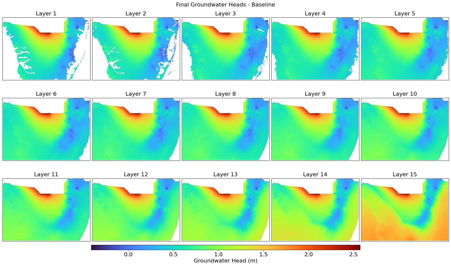
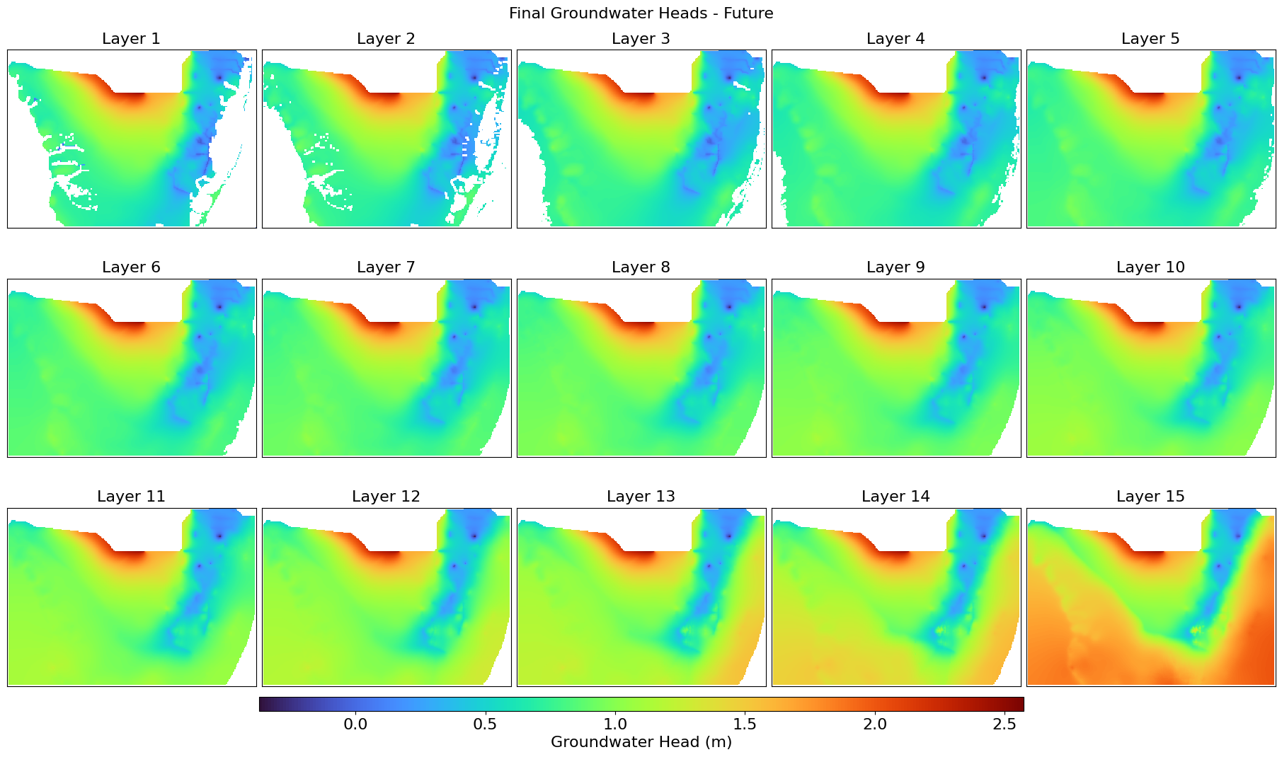
This script extracts, compares, and visualizes groundwater head distributions from BISECT .uhd output files for the final stress period. It reads 3D head data, filters inactive cells, and generates layer-wise GeoTIFFs and comparison maps for baseline and future scenarios. The difference in head values is also computed and visualized using color stretches over a UTM-projected grid.
import flopy.utils.binaryfile as bf
import numpy as np
import rasterio
from rasterio.transform import from_origin
import matplotlib.pyplot as plt
import os
import matplotlib.colors as mcolors
def extract_heads_final(udh_file, final_stress_period=3286):
"""
Extracts the spatial grid of head values for the final stress period,
while treating -9999 values as inactive cells.
"""
head_obj = bf.HeadFile(udh_file)
heads_3d = head_obj.get_data(totim=final_stress_period)
# Convert unwanted values (-9999) to NaN
heads_3d = np.where(heads_3d == 999, np.nan, heads_3d)
return heads_3d
def save_heads_layers_as_tiff(heads_3d, output_folder, prefix, left, right, top, bottom):
"""
Saves each groundwater head layer as a separate GeoTIFF file.
"""
os.makedirs(output_folder, exist_ok=True)
nrows, ncols = heads_3d.shape[1], heads_3d.shape[2]
cell_width = (right - left) / ncols
cell_height = (top - bottom) / nrows
transform = from_origin(left, top, cell_width, cell_height)
for i in range(heads_3d.shape[0]):
output_path = os.path.join(output_folder, f"{prefix}_Layer_{i+1}.tif")
meta = {
'driver': 'GTiff',
'dtype': 'float32',
'nodata': np.nan,
'width': ncols,
'height': nrows,
'count': 1,
'crs': 'EPSG:26917',
'transform': transform
}
with rasterio.open(output_path, 'w', **meta) as dst:
dst.write(heads_3d[i, :, :].astype(np.float32), 1)
#print(f"Saved: {output_path}")
def plot_heads_layers(heads_3d, title, output_file, left, right, top, bottom):
"""
Displays all groundwater head layers with a percent clip stretch type.
"""
fig, axes = plt.subplots(nrows=3, ncols=5, figsize=(18, 10), constrained_layout=True)
extent = [left, right, bottom, top]
vmin, vmax = np.nanpercentile(heads_3d, [0, 100]) # Percent clip stretch (0.5%-99.9%)
cmap = plt.get_cmap("turbo")
norm = mcolors.Normalize(vmin=vmin, vmax=vmax)
for i, ax in enumerate(axes.flat):
if i < heads_3d.shape[0]:
img = ax.imshow(heads_3d[i, :, :], extent=extent, cmap=cmap, origin='upper', norm=norm)
ax.set_title(f'Layer {i+1}', fontsize=16)
ax.set_xticks([])
ax.set_yticks([])
cbar_ax = fig.add_axes([0.2, 0.001, 0.6, 0.02])
cbar = fig.colorbar(img, cax=cbar_ax, orientation='horizontal')
cbar.set_label('Groundwater Head (m)', fontsize=16)
cbar.ax.tick_params(labelsize=16)
plt.suptitle(title, fontsize=16)
plt.savefig(output_file, dpi=300, bbox_inches='tight')
plt.show()
# File paths
baseline_udh = "C:/Users/mgebremedhin/Documents/FGCU/BISECT/Model_new/Baseline/output/Output.Baseline/timeBB.uhd"
future_udh = "C:/Users/mgebremedhin/Documents/FGCU/BISECT/Model_new/nearFuture/output/Output.Future/timeBB.uhd"
output_folder = "C:/Users/mgebremedhin/Documents/FGCU/BISECT/PostProcessing/GW_Heads/Tiff_Final"
# Define bounding box
left, right, top, bottom = 461000.0, 590500.0, 2872000.0, 2779000.0
# Extract heads for final stress period
heads_baseline_final = extract_heads_final(baseline_udh)
heads_future_final = extract_heads_final(future_udh)
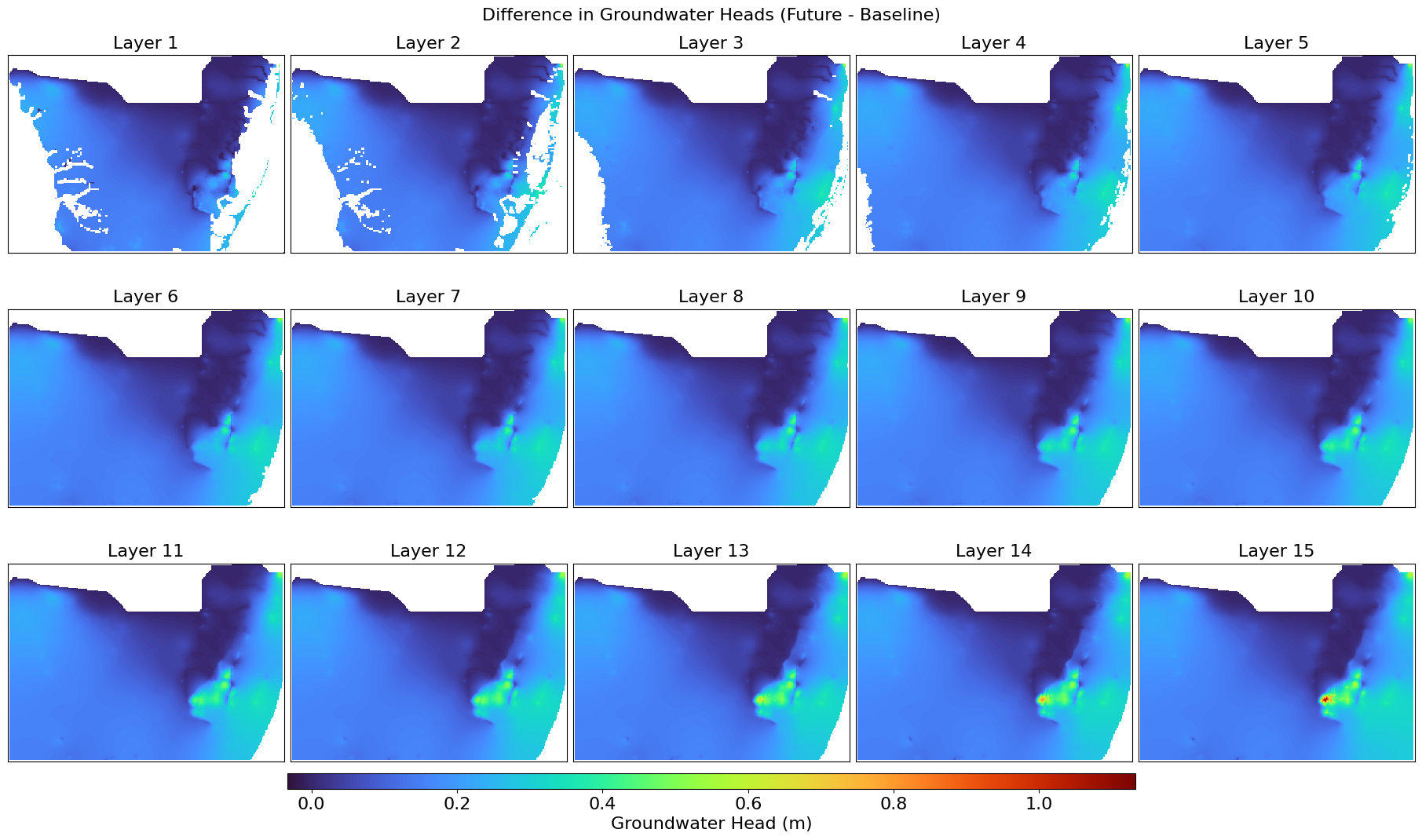
# Compute difference (Future - Baseline)
heads_difference = heads_future_final - heads_baseline_final
# Save each layer as a TIFF file
save_heads_layers_as_tiff(heads_baseline_final, output_folder, "Heads_Baseline_Final", left, right, top, bottom)
save_heads_layers_as_tiff(heads_future_final, output_folder, "Heads_Future_Final", left, right, top, bottom)
save_heads_layers_as_tiff(heads_difference, output_folder, "Heads_Difference_Final", left, right, top, bottom)
# Display all layers
plot_heads_layers(heads_baseline_final, "Final Groundwater Heads - Baseline",
"Heads_Baseline_Final.png",
left, right, top, bottom)
plot_heads_layers(heads_future_final, "Final Groundwater Heads - Future",
"Heads_Future_Final.png",
left, right, top, bottom)
plot_heads_layers(heads_difference, "Difference in Groundwater Heads (Future - Baseline)",
"Heads_Difference_Final.png",
left, right, top, bottom)
This script extracts time series salinity (concentration) data from a BISECT simulated MT3D .UCN binary file for a specified grid cell across all vertical layers. It compiles the values into a pandas DataFrame with timestamps and per-layer salinity, enabling export to CSV for further analysis.
import flopy.utils.binaryfile as bf
import pandas as pd
import numpy as np

def extract_salinity_timeseries(ucn_file, col, row):
    """
    Extracts the salinity (concentration) values for all layers at a given column and row.

    Parameters:
        ucn_file (str): Path to the MT3D UCN binary file.
        col (int): Column index.
        row (int): Row index.

    Returns:
        pd.DataFrame: DataFrame containing Time and Salinity values for each layer.
    """
    # Load the UCN file
    ucn_obj = bf.UcnFile(ucn_file)

    # Get simulation times
    times = ucn_obj.get_times()

    # Initialize list to store salinity values
    salinity_data = []

    for t in times:
        conc = ucn_obj.get_data(totim=t)  # 3D array of concentrations at this time step

        # Extract values from each layer at the given row, col
        layer_values = [conc[layer, row, col] for layer in range(conc.shape[0])]

        # Append time and salinity values
        salinity_data.append([t] + layer_values)

    # Create column names dynamically for all layers
    layer_columns = [f"Layer_{i+1}" for i in range(conc.shape[0])]

    # Create DataFrame
    df = pd.DataFrame(salinity_data, columns=["Time"] + layer_columns)

    return df

# Example Usage
ucn_file = "C:/Users/mgebremedhin/Documents/FGCU/BISECT/Model_new/Baseline/output/Output.Baseline/MT3D001.UCN"

# Specify row and column
col, row = 184, 144  # Example grid coordinates

# Extract salinity data for all layers
salinity_df = extract_salinity_timeseries(ucn_file, col, row)

# Display the first few rows
print(salinity_df.head())

# Save to CSV (optional)
output_file = f"C:/Users/mgebremedhin/Documents/FGCU/BISECT/PostProcessing/BISECT_Validation/Salinity_timeseries_Baseline_grid_{col}_{row}.csv"
salinity_df.to_csv(output_file, index=False)
#print(f"Saved CSV successfully: {output_file}")
   Time   Layer_1   Layer_2   Layer_3   Layer_4   Layer_5   Layer_6   Layer_7  \
0   1.0  0.679733  0.772024  1.338979  2.337256  3.610289  5.077246  6.852144
1   2.0  0.679552  0.771788  1.339062  2.337384  3.610240  5.077137  6.851869
2   3.0  0.679279  0.773035  1.341798  2.340626  3.613560  5.080600  6.855250
3   4.0  0.679847  0.776326  1.348086  2.348184  3.621765  5.089721  6.864512
4   5.0  0.680758  0.779984  1.354956  2.357055  3.631710  5.100378  6.874903

    Layer_8    Layer_9   Layer_10   Layer_11   Layer_12   Layer_13   Layer_14  \
0  8.962332  11.327460  13.878865  16.679836  20.196846  21.343370  21.453350
1  8.961963  11.327412  13.878721  16.679436  20.196201  21.343332  21.453348
2  8.965066  11.329945  13.880394  16.680258  20.196302  21.343332  21.453354
3  8.973144  11.336127  13.884745  16.682961  20.196623  21.343348  21.453398
4  8.982054  11.342890  13.889488  16.685915  20.197044  21.343367  21.453440

    Layer_15
0  22.400387
1  22.400394
2  22.400408
3  22.400429
4  22.400450
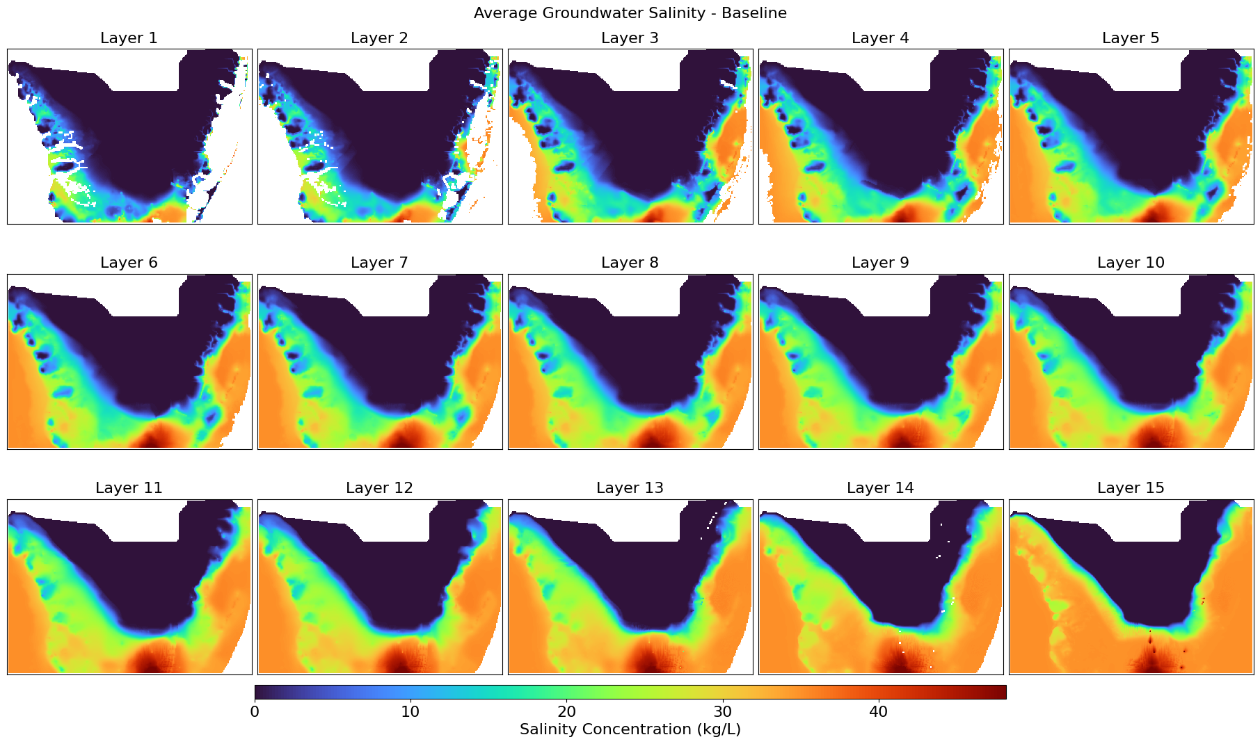
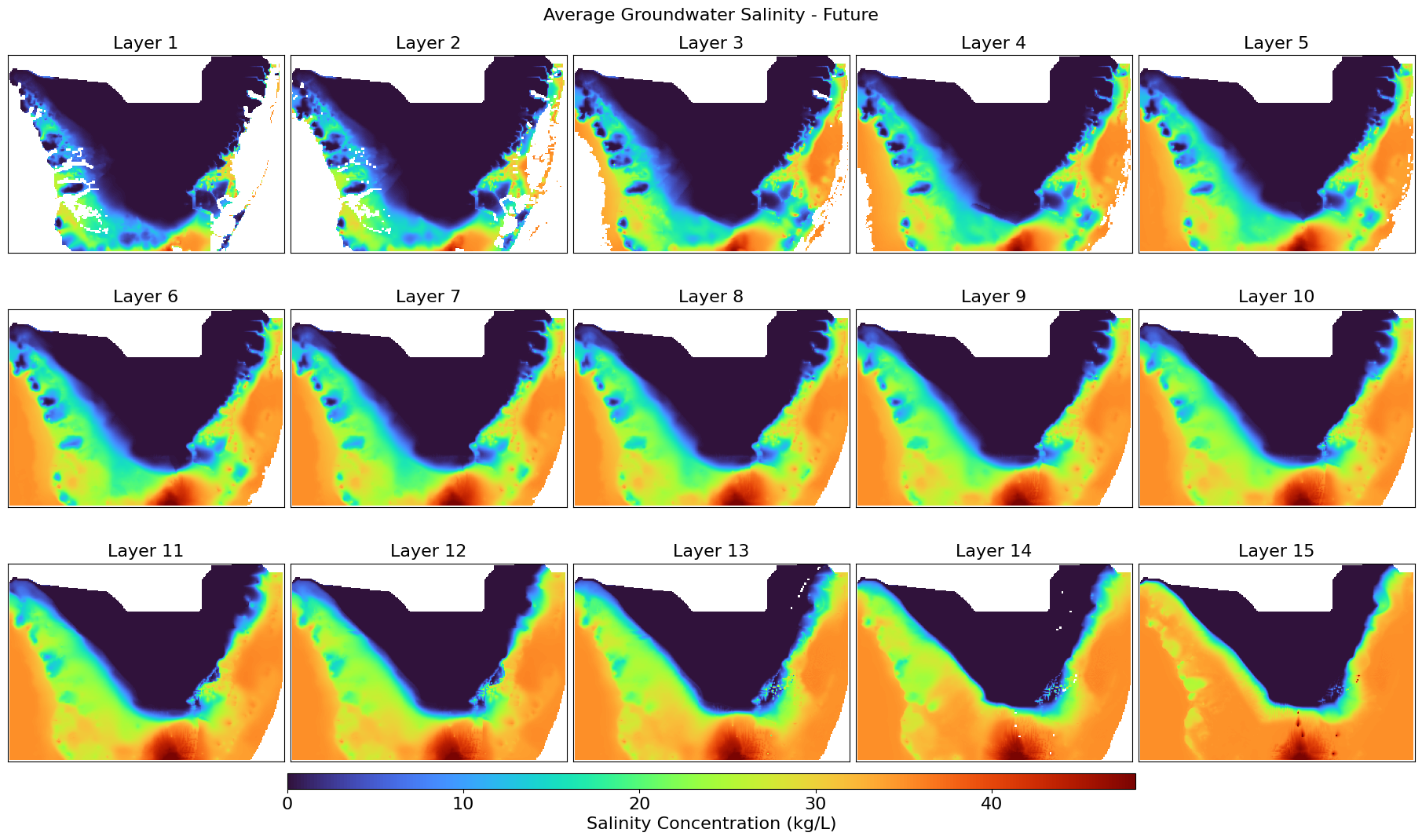
This script calculates the average groundwater salinity across all stress periods from MT3D .UCN files and visualizes the spatial distribution per layer. It exports the averaged salinity layers as GeoTIFFs and generates color visual plots for both baseline and future scenarios, along with their difference, mapped over a defined UTM-projected extent.
import flopy.utils.binaryfile as bf
import numpy as np
import rasterio
from rasterio.transform import from_origin
import matplotlib.pyplot as plt
import os
import matplotlib.colors as mcolors
def extract_salinity_avg(ucn_file):
"""
Extracts and computes the average salinity across all stress periods.
"""
ucn_obj = bf.UcnFile(ucn_file)
times = ucn_obj.get_times()
salinity_list = [ucn_obj.get_data(totim=t) for t in times]
salinity_3d_avg = np.nanmean(np.where(np.isin(salinity_list, [-9999, 999, -1]), np.nan, salinity_list), axis=0)
return salinity_3d_avg
def save_salinity_layers_as_tiff(salinity_3d, output_folder, prefix, left, right, top, bottom):
"""
Saves each groundwater salinity layer as a separate GeoTIFF file.
"""
os.makedirs(output_folder, exist_ok=True)
nrows, ncols = salinity_3d.shape[1], salinity_3d.shape[2]
cell_width = (right - left) / ncols
cell_height = (top - bottom) / nrows
transform = from_origin(left, top, cell_width, cell_height)
for i in range(salinity_3d.shape[0]):
output_path = os.path.join(output_folder, f"{prefix}_Layer_{i+1}.tif")
meta = {
'driver': 'GTiff',
'dtype': 'float32',
'nodata': np.nan,
'width': ncols,
'height': nrows,
'count': 1,
'crs': 'EPSG:26917',
'transform': transform
}
with rasterio.open(output_path, 'w', **meta) as dst:
dst.write(salinity_3d[i, :, :].astype(np.float32), 1)
def plot_salinity_layers(salinity_3d, title, output_file, left, right, top, bottom):
"""
Displays all groundwater salinity layers with a percent clip stretch type.
"""
fig, axes = plt.subplots(nrows=3, ncols=5, figsize=(18, 10), constrained_layout=True)
extent = [left, right, bottom, top]
vmin, vmax = np.nanpercentile(salinity_3d, [0.5, 99.9])
cmap = plt.get_cmap("turbo")
norm = mcolors.Normalize(vmin=vmin, vmax=vmax)
for i, ax in enumerate(axes.flat):
if i < salinity_3d.shape[0]:
img = ax.imshow(salinity_3d[i, :, :], extent=extent, cmap=cmap, origin='upper', norm=norm)
ax.set_title(f'Layer {i+1}', fontsize=16)
ax.set_xticks([])
ax.set_yticks([])
cbar_ax = fig.add_axes([0.2, 0.001, 0.6, 0.02])
cbar = fig.colorbar(img, cax=cbar_ax, orientation='horizontal')
cbar.set_label('Salinity Concentration (kg/L)', fontsize=16)
cbar.ax.tick_params(labelsize=16)
plt.suptitle(title, fontsize=16)
plt.savefig(output_file, dpi=300, bbox_inches='tight')
plt.show()
# File paths
baseline_ucn = "C:/Users/mgebremedhin/Documents/FGCU/BISECT/Model_new/Baseline/output/Output.Baseline/MT3D001.UCN"
future_ucn = "C:/Users/mgebremedhin/Documents/FGCU/BISECT/Model_new/FarFuture/output/Output.Future/MT3D001.UCN"
output_folder = "C:/Users/mgebremedhin/Documents/FGCU/BISECT/PostProcessing/GW_Salinity/Tiff_Final"
# Define bounding box
left, right, top, bottom = 461000.0, 590500.0, 2872000.0, 2779000.0
# Extract average salinity over all stress periods
salinity_baseline_avg = extract_salinity_avg(baseline_ucn)
salinity_future_avg = extract_salinity_avg(future_ucn)
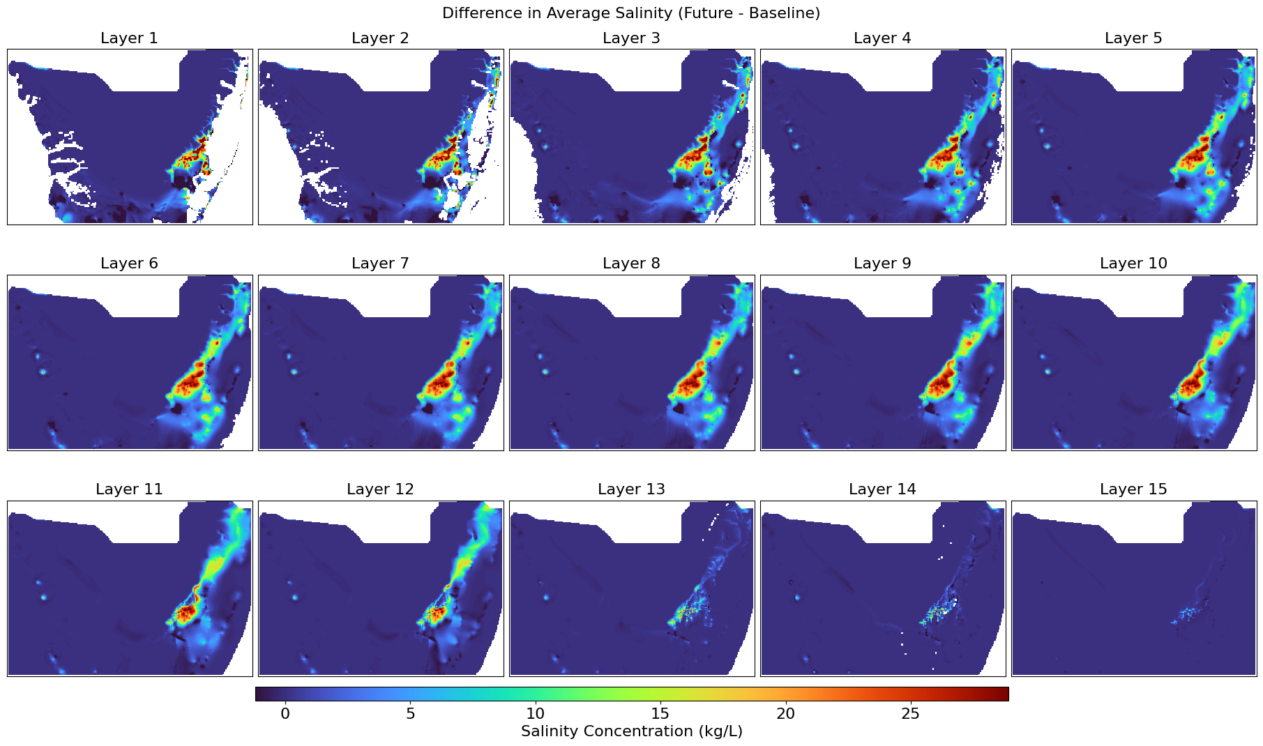
# Compute difference (Future - Baseline)
salinity_difference = salinity_future_avg - salinity_baseline_avg
# Save each layer as a TIFF file
save_salinity_layers_as_tiff(salinity_baseline_avg, output_folder, "Salinity_Baseline_Avg", left, right, top, bottom)
save_salinity_layers_as_tiff(salinity_future_avg, output_folder, "Salinity_Future_Avg", left, right, top, bottom)
save_salinity_layers_as_tiff(salinity_difference, output_folder, "Salinity_Difference_Avg", left, right, top, bottom)
# Display all layers
plot_salinity_layers(salinity_baseline_avg, "Average Groundwater Salinity - Baseline",
"Salinity_Baseline_Avg.png",
left, right, top, bottom)
plot_salinity_layers(salinity_future_avg, "Average Groundwater Salinity - Future",
"Salinity_FarFuture_Avg.png",
left, right, top, bottom)
plot_salinity_layers(salinity_difference, "Difference in Average Salinity (Future - Baseline)",
"Salinity_Difference_Avg.png",
left, right, top, bottom)